 G-Cubed
Choose a chart type
Choose a chart to answer an economic question: how an outcome evolves, how regions compare, or how simulation layers contribute to an experiment’s result. Start with the real model-run examples: GDP and inflation paths, regional GDP bars and sector-output panels from a saved 2A baseline. Use lines when the timing of an adjustment matters. For experiment results, prefer selected-year deviation bars and heatmaps centred on zero; use compositions and waterfalls only with suitable additive data.
A series is one row of observations in the projections CSV, such as inflation in the USA. A dimension is a model set, such as regions or sectors. Its members are the codes in that set. A chartpack selects these rows and their presentation; it does not run an experiment or calculate new model results.
| Economic question | Chart type | YAML setting |
|---|---|---|
| How does an outcome evolve? | Line | Omit chart_type |
| How much does it change between two years? | Change between years | chart_type: series-delta |
| How do regions or sectors compare in one year? | Single-year bars | chart_type: series-value |
| Where are outcomes high or low across sets and years? | Heatmap | chart_type: heatmap |
| How do many time paths compare? | Small multiples | chart_type: small-multiples |
| How do two measures relate? | Paired scatter | chart_type: paired-scatter |
| How do parts of a total change over time? | Stacked areas | chart_type: composition-area |
| What shares make up a total? | Stacked bars | chart_type: composition-bar |
| How do ordered simulation layers lead to the final result? | Waterfall | chart_type: waterfall |
Explore the chart types
The 11 charts below and their YAML are copied from the latest template builder’s chart-types guide, reviewed on 25 September 2026. All observations are synthetic. Names beginning with SYNTH are teaching examples, not built-in G-Cubed variables. The regional labels are illustrative too.
Download all example chart declarations and the matching sample CSV. Each chart also has its own complete YAML download. Use the same sample CSV with any individual example. Titles, plots and captions below follow the report card order.
Open the interactive chart guide to explore 22 rendered states, including Year, View, Observations and Display previews. Save that self-contained page to use it offline. Its preview selectors swap pre-rendered SVGs; a generated report recalculates its charts, tables and exports. Preview Axes is an authoring demonstration, not a report dropdown: change x_dimension and y_dimension in YAML to transpose a heatmap. The YAML downloads describe each chart’s initial state.
To assemble a chartpack from the entries shown below, begin with this header once, then add your chosen - chart: entries in presentation order:
- chartpack:
    format: gcubed-chartpack
    version: "1.4.0"
    title: Illustrative experiment results
    sector_selection_dimensions: [sectors, layers]
    defaults:
      start_year: 2025
      end_year: 2035
This header uses dimensions present in the sample CSV. For a real experiment, replace the SYNTH names, dimensions, years, captions and units with those in your own results. Omit sector_selection_dimensions if you want the usual sector and goods choices. Copy the standalone declarations into a chartpack file, rather than into the differently structured setup.yaml.
These examples use chartpack "1.4.0". Lines are available in every supported version; delta bars were added in "1.2.0". The other types and the newer controls require 1.4 support. Check both the reporting package and the report template.
Show a trend with lines
Each line follows one region through time. The example uses an activity index with 2025 equal to 100. Its level shows activity relative to that reference year; it is not a percentage deviation from a G-Cubed baseline.
Leave out chart_type; chart_type: line is not an accepted declaration. Selected series must have common units. Missing observations remain gaps.
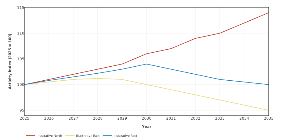
Synthetic regional activity paths use complete annual observations; real gaps remain gaps.
- chart:
    title: Illustrative activity paths
    caption: Synthetic regional activity paths use complete annual observations; real gaps remain gaps.
    x_axis:
      label: Year
    y_axis:
      label: Activity index (2025 = 100)
    series:
    - variable: SYNTHINDEX(USA)
      label: Illustrative North
    - variable: SYNTHINDEX(JPN)
      label: Illustrative East
    - variable: SYNTHINDEX(ROW)
      label: Illustrative Rest
Download this complete chartpack · Download the matching sample CSV.
Change between two years
The bar for each region is its 2035 index minus its 2025 index. Teal marks an increase, rust a decrease, and the neutral colour marks zero. These are index-point changes, not growth rates. The chart inherits its two years from the header above and sorts bars from the largest change to the smallest.
With experiment deviation data, the same declaration shows the change in the deviation between two years. For example, a GDP deviation moving from −2% to −1% gives a difference of +1 percentage point. To show the deviation in 2035 itself, use the single-year chart below.
All bars must share a variable prefix, units and ordered dimensions, varying across at most one set. Both endpoint values must be available. See delta endpoints to use different years for one bar.
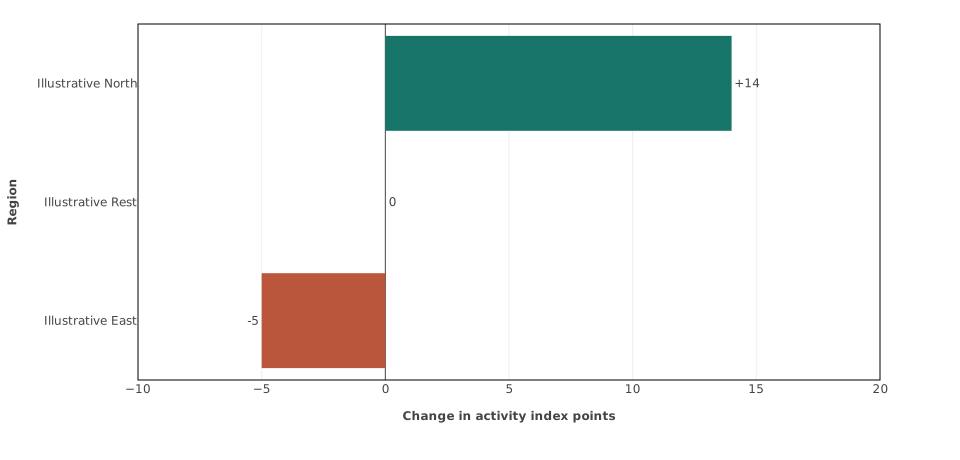
Teal marks positive change, rust negative change, and neutral zero; labels retain the authored units.
- chart:
    title: Activity change, 2025–2035
    chart_type: series-delta
    show_labels: true
    color_by_sign: true
    caption: Teal marks positive change, rust negative change, and neutral zero; labels retain the authored units.
    orientation: horizontal
    sort: value-descending
    x_axis:
      label: Change in activity index points
      min: -10
      max: 20
    y_axis:
      label: Region
    series:
    - variable: SYNTHINDEX(USA)
      label: Illustrative North
    - variable: SYNTHINDEX(JPN)
      label: Illustrative East
    - variable: SYNTHINDEX(ROW)
      label: Illustrative Rest
Download this complete chartpack · Download the matching sample CSV.
Compare values in one year
These bars compare sector output in 2030, measured in US$ billion at 2025 prices. year chooses the initial year. Bars are horizontal by default; sort: value-descending places larger values first. A Year control appears when at least two eligible years are available.
On a baseline-deviation CSV, this chart instead shows each series’ deviation from baseline in the selected year. Its units come from that CSV. Series must share units, but may have different prefixes and dimension structures.
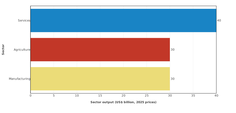
A report card offers every eligible year and refreshes its title, table, and exports together.
- chart:
    title: Illustrative North sector output in 2030
    chart_type: series-value
    show_labels: true
    year: 2030
    caption: A report card offers every eligible year and refreshes its title, table, and exports together.
    sort: value-descending
    x_axis:
      label: Sector output (US$ billion, 2025 prices)
      min: 0
    y_axis:
      label: Sector
    series:
    - variable_prefix: SYNTHSECTOR
      selectors:
        sectors: all
        regions: USA
Download this complete chartpack · Download the matching sample CSV.
Compare two dimensions in a heatmap
A heatmap uses colour to show values. In this first example, rows are regions and columns are years. The neutral colour marks the reference index value of
- A midpoint changes the colour scale; it does not convert observations into indices, shares or deviations.
Use different x_dimension and y_dimension keys. Selected rows must share one prefix, units and ordered dimensions; every dimension outside the axes must stay fixed. Missing observations leave blank cells, while zero remains a value. Duplicate cells are invalid: the chart does not add them together. A time-axis heatmap cannot have a chart-level year or year_selector.
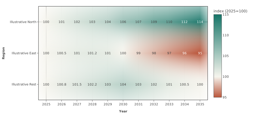
A semantic diverging palette anchors the authored midpoint; a time-axis heatmap has no Year control.
- chart:
    title: Activity by region and year
    chart_type: heatmap
    show_labels: true
    x_dimension: year
    y_dimension: regions
    x_axis:
      label: Year
    y_axis:
      label: Region
    color_axis:
      min: 95
      max: 115
      midpoint: 100
      palette: semantic-diverging
    caption: A semantic diverging palette anchors the authored midpoint; a time-axis heatmap has no Year control.
    series:
    - variable_prefix: SYNTHINDEX
      selectors:
        regions: all
Download this complete chartpack · Download the matching sample CSV.
Compare regions and sectors in one year
This second heatmap places regions on one axis and sectors on the other. With two model dimensions, year is required. year_selector: true lets the reader choose another eligible year. The pale-to-teal scale suits these nonnegative output levels.
The report’s table follows the same row-and-column layout. Related heatmaps can share a View control; see heatmap colours and views.
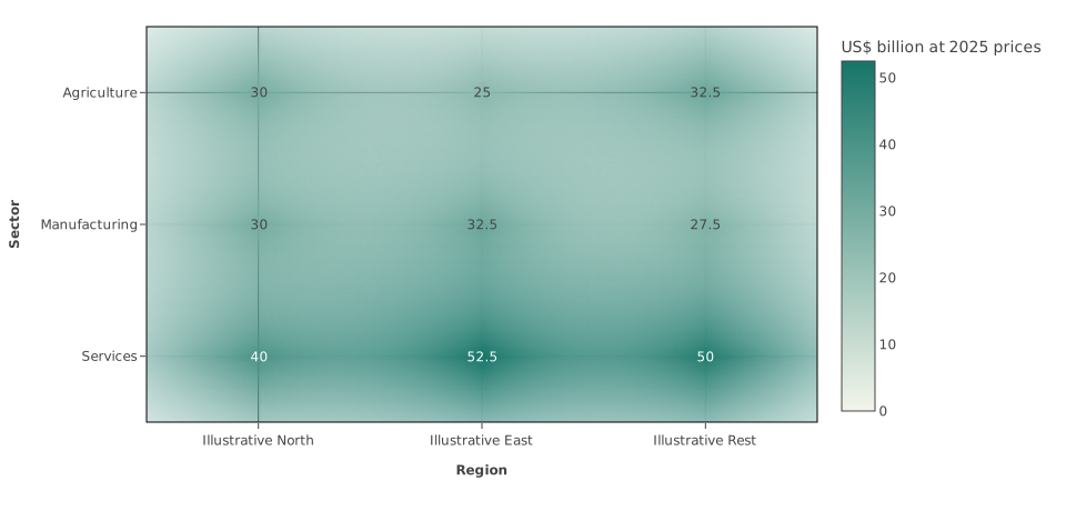
Two model dimensions form a matrix; the report Year control retains the authored measure and bounds.
- chart:
    title: Sector output by region in 2030
    chart_type: heatmap
    show_labels: true
    x_dimension: regions
    y_dimension: sectors
    x_axis:
      label: Region
    y_axis:
      label: Sector
    year: 2030
    year_selector: true
    color_axis:
      min: 0
      palette: semantic-sequential
    caption: Two model dimensions form a matrix; the report Year control retains the authored measure and bounds.
    series:
    - variable_prefix: SYNTHSECTOR
      selectors:
        sectors: all
        regions: all
Download this complete chartpack · Download the matching sample CSV.
Switch between related heatmap views
Open the grouped View example and download its complete chartpack. Use the same sample CSV.
The first view puts years on an axis. The second uses regions and sectors, so it offers a separate Year control. Each view retains its own measure, units and colour scale: the first shows an activity index, the second output levels. Switching View does not convert one measure into the other. The two adjacent chart definitions share view_group and have distinct view_label values. See the grouping rules.
Give each member its own small chart
Each region receives a panel, with a line for each sector. All panels share the same year and value scales, making differences in both size and timing comparable. This helps when a single plot would have too many lines.
facet_dimension selects the set used to separate panels. The optional group_dimension selects the lines within each panel. Both must be different model dimensions. Rows must share one prefix, units and ordered dimensions; other dimensions must stay fixed. A sector keeps the same colour across panels. Missing observations remain gaps.
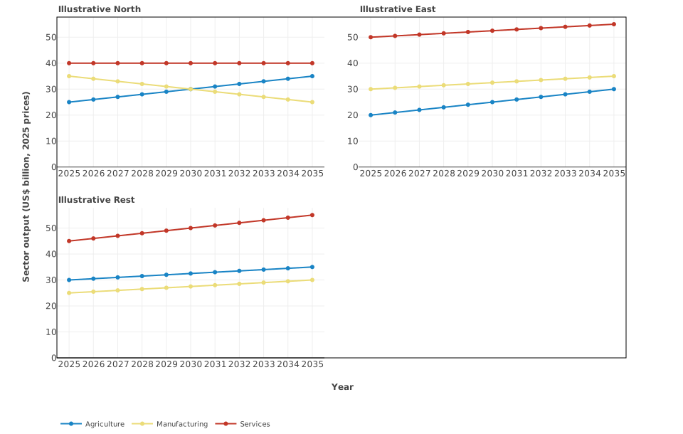
Small multiples share time and value scales so magnitude and shape remain comparable across facets.
- chart:
    title: Sector output paths by region
    chart_type: small-multiples
    facet_dimension: regions
    group_dimension: sectors
    x_axis:
      label: Year
    y_axis:
      label: Sector output (US$ billion, 2025 prices)
      min: 0
    caption: Small multiples share time and value scales so magnitude and shape remain comparable across facets.
    series:
    - variable_prefix: SYNTHSECTOR
      selectors:
        sectors: all
        regions: all
Download this complete chartpack · Download the matching sample CSV.
Compare two measures
Each point pairs a region’s activity index with its emissions in 2030. The X and Y axes have different units: an index and Mt CO2-e. This plot shows association; it does not establish that one outcome causes the other.
Write each pair using exact x_variable and y_variable names. Selectors cannot create these pairs. Both values must be available in the selected year, and shared dimensions must use the same member: pair USA activity with USA emissions. A dimension used on only one axis, such as a gas, must stay fixed across pairs. All X observations share one unit; all Y observations share another. The Year control moves the pairs together.
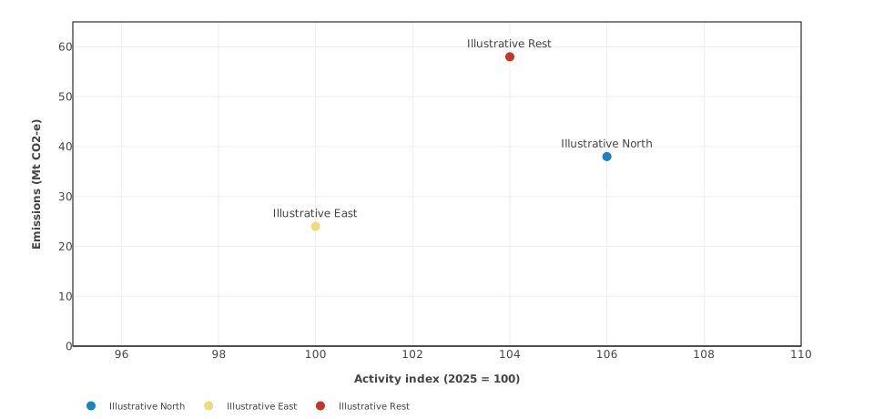
A report Year control moves every complete regional X/Y pair together while preserving fixed axes.
- chart:
    title: Activity and emissions in 2030
    chart_type: paired-scatter
    show_labels: true
    year: 2030
    year_selector: true
    caption: A report Year control moves every complete regional X/Y pair together while preserving fixed axes.
    x_axis:
      label: Activity index (2025 = 100)
      min: 95
      max: 110
    y_axis:
      label: Emissions (Mt CO2-e)
      min: 0
      max: 65
    series:
    - x_variable: SYNTHINDEX(USA)
      y_variable: SYNTHEMISSIONS(USA)
      label: Illustrative North
    - x_variable: SYNTHINDEX(JPN)
      y_variable: SYNTHEMISSIONS(JPN)
      label: Illustrative East
    - x_variable: SYNTHINDEX(ROW)
      y_variable: SYNTHEMISSIONS(ROW)
      label: Illustrative Rest
Download this complete chartpack · Download the matching sample CSV.
Follow two measures through time
With exactly one pair, observation_mode: selectable begins with its path through time. The plotted points use existing annual observations in the selected range, connected in chronological order. Years lacking either value are omitted; no missing values are estimated. Connections do not establish causality.
The Observations control switches between Across years and Single year. year is still required for the single-year view. Do not combine this mode with year_selector: false.
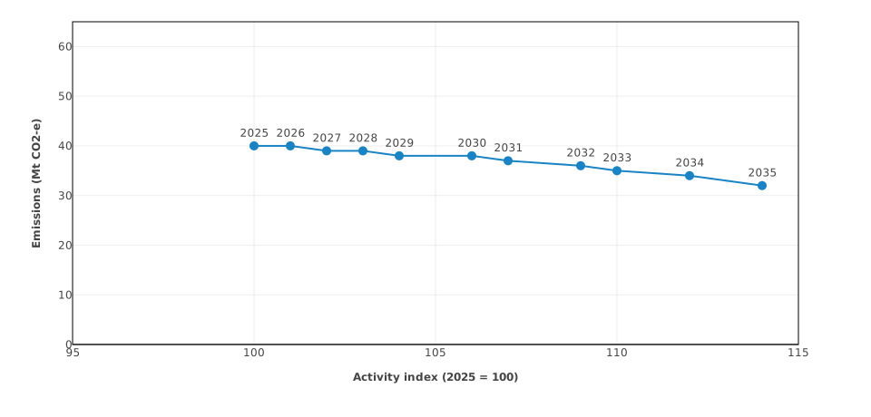
Across years connects existing annual observations chronologically; Single year restores the authored point.
- chart:
    title: Illustrative North activity and emissions trajectory
    chart_type: paired-scatter
    show_labels: true
    year: 2030
    observation_mode: selectable
    x_axis:
      label: Activity index (2025 = 100)
      min: 95
      max: 115
    y_axis:
      label: Emissions (Mt CO2-e)
      min: 0
      max: 65
    caption: Across years connects existing annual observations chronologically; Single year restores the authored point.
    series:
    - x_variable: SYNTHINDEX(USA)
      y_variable: SYNTHEMISSIONS(USA)
      label: Illustrative North
Download this complete chartpack · Download the matching sample CSV.
Show parts of a total over time
The stacked areas show sector output adding to a sector output total in each year. Gross sector output is not a decomposition of GDP: intermediate production is included. Use the measure and price basis appropriate to the economic question.
reconciliation.total_variable identifies the row containing the total. Components must be complete, nonnegative, use common units and a common prefix and ordered dimensions, and vary across at most one set. The total must have the same units and regional coverage. They must add up in every displayed year; the example’s zero tolerance requires exact equality.
display_selector: true offers stacked areas or bars. Hiding components produces a partial-composition notice. Percentage deviations from baseline are not additive components. Prepare suitable levels or shares before making this chart; see choosing report data.
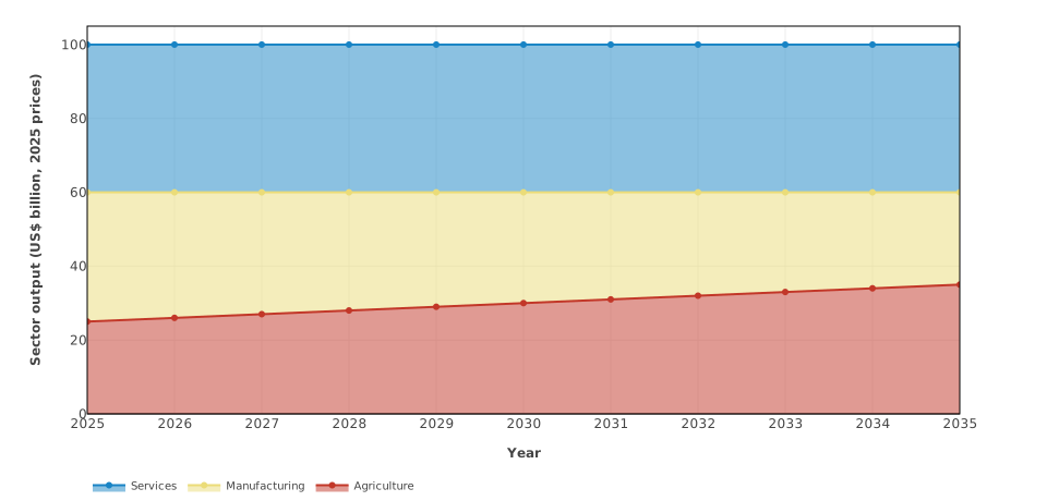
Complete additive levels reconcile to the authored total; Display switches area and bars without changing data.
- chart:
    title: Illustrative North sector output total
    chart_type: composition-area
    show_labels: true
    display_selector: true
    x_axis:
      label: Year
    y_axis:
      label: Sector output (US$ billion, 2025 prices)
      min: 0
    caption: Complete additive levels reconcile to the authored total; Display switches area and bars without changing data.
    reconciliation:
      total_variable: SYNTHTOTAL(USA)
      absolute_tolerance: 0
    series:
    - variable_prefix: SYNTHSECTOR
      selectors:
        sectors: all
        regions: USA
Download this complete chartpack · Download the matching sample CSV.
Show parts of a total as bars
The example begins with one stacked bar for 2035. Its component shares are already percentages that add to 100; reconciliation.total: 100 checks that sum. The template does not calculate or normalise shares.
Use year together with year_selector: true to begin with one year and allow selection of other valid years. Without year, compositions show their whole start-to-end range, even if a Year control is enabled. A fixed single-year bar can also use equal start_year and end_year bounds. The same completeness and additivity rules apply as for stacked areas.
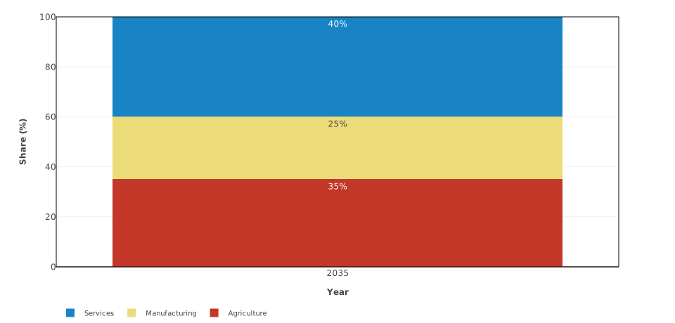
Choose one eligible year and either stacked display; the synthetic shares continue to reconcile to 100 percent.
- chart:
    title: Illustrative North sector output shares in 2035
    chart_type: composition-bar
    show_labels: true
    year: 2035
    year_selector: true
    display_selector: true
    x_axis:
      label: Year
    y_axis:
      label: Share (%)
      min: 0
      max: 100
    caption: Choose one eligible year and either stacked display; the synthetic shares continue to reconcile to 100 percent.
    reconciliation:
      total: 100
      absolute_tolerance: 0
    series:
    - variable_prefix: SYNTHSHARE
      selectors:
        sectors: all
        regions: USA
Download this complete chartpack · Download the matching sample CSV.
Explain a change step by step
The waterfall shows how ordered simulation layers bridge the baseline and the final experiment result in 2030. Its synthetic contributions satisfy 0 − 12 − 9 + 10 + 3 = −8, in US$ billion at 2025 prices.
Use one start, then one or more contribution entries, then one total. Contributions must be changes from each immediately preceding simulation layer, expressed in common additive units. Adding each layer’s cumulative deviation from baseline would count earlier effects more than once. The allocation of contributions depends on the order of the layers.
The source CSV must already contain these contribution rows. A selector retains CSV row order; use exact variables in the required order when that order differs. All nonblank region metadata must agree. The complete sequence must add to its stated total; one missing or invalid step rejects the chart. Filters hide the whole waterfall rather than leaving a partial decomposition.
The sample provides complete contributions for 2025 and 2030, so its Year control offers both years. The 2025 contributions reconcile as 0 − 10 − 7 + 8 + 3 = −6. Other years have missing contributions and are not offered. Try both years in the waterfall preview.
Here level_base: 100 adds 100 to the cumulative change in the visible table’s Level column. It requires a zero start and leaves the plotted changes and CSV unchanged. For an experiment, use the appropriate baseline level in the same units. See preparing layer contributions.
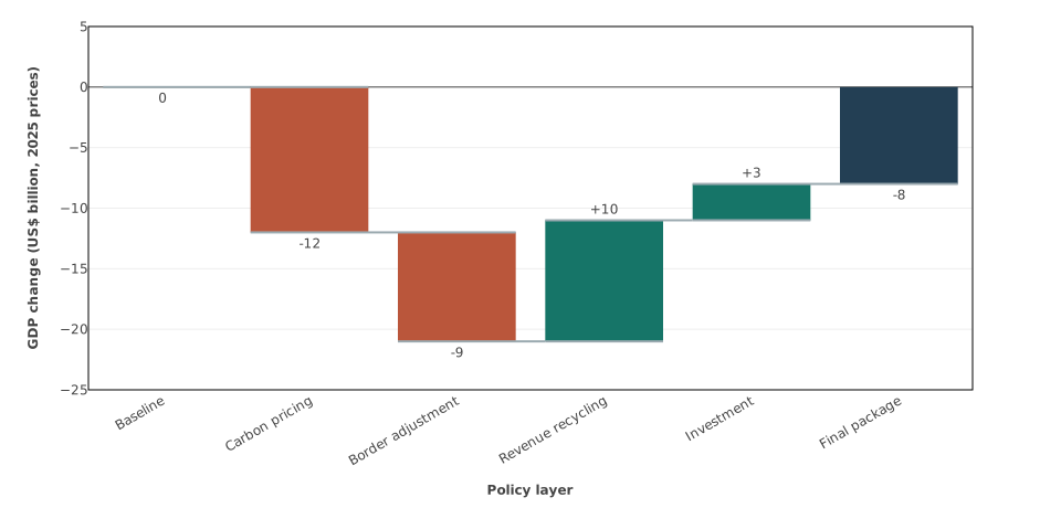
Ordered contributions reconcile from zero; the report table derives an absolute level from base 100.
- chart:
    title: Ordered policy-layer contribution in 2030
    chart_type: waterfall
    show_labels: true
    year: 2030
    year_selector: true
    level_base: 100
    caption: Ordered contributions reconcile from zero; the report table derives an absolute level from base 100.
    x_axis:
      label: Policy layer
    y_axis:
      label: GDP change (US$ billion, 2025 prices)
      min: -25
      max: 5
    series:
    - variable: SYNTHGDPCHANGE(BASELINE,USA)
      label: Baseline
      role: start
    - variable_prefix: SYNTHGDPCONTRIBUTION
      selectors:
        regions: USA
      role: contribution
    - variable: SYNTHGDPCHANGE(PACKAGE,USA)
      label: Final package
      role: total
Download this complete chartpack · Download the matching sample CSV.
Continue with your experiment
Use display options for captions, labels, colours and report controls, and validation and troubleshooting when a chart does not appear. Alternative deterministic experiments are not uncertainty intervals; fan charts are not part of this release.